Abstract
To fix ideas
We present an introduction to the solution of multi-stage optimization problems. Starting from the dynamic programming algorithm, we consider theoretical and computational aspects, mainly of deterministic problems, and discuss how to generalize some of the results to Markovian decision processes.
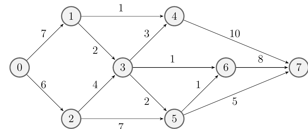
| Path | Cost |
|---|---|
| \(0 \to 1 \to 4 \to 7\) | 18 |
| \(0 \to 1 \to 3 \to 4 \to 7\) | 22 |
| \(0 \to 1 \to 3 \to 6 \to 7\) | 18 |
| \(0 \to 1 \to 3 \to 5 \to 6 \to 7\) | 20 |
| \(\mathbf{0 \to 1 \to 3 \to 5 \to 7}\) | 16 |
| \(0 \to 2 \to 3 \to 4 \to 7\) | 23 |
| \(0 \to 2 \to 3 \to 6 \to 7\) | 19 |
| \(0 \to 2 \to 3 \to 5 \to 6 \to 7\) | 21 |
| \(0 \to 2 \to 3 \to 5 \to 7\) | 17 |
| \(0 \to 2 \to 5 \to 6 \to 7\) | 22 |
| \(0 \to 2 \to 5 \to 7\) | 18 |
The classic problem with which the essential ideas of dynamic programming can be introduced is the optimal route problem (shortest route considering distances,or cheapest route considering costs) [1,2]. A simple version of this problem is shown schematically in Figure fig-brandimarte_net. By exhaustion, we deploy the cost of path in Table tbl-brandimarte_paths.
In this problem, the optimal route to go from the node labeled \(0\) to the node labeled \(7\) is to be determined. The costs between each pair of nodes connected by an arrow are represented by a number next to it. For example, the cost to go from node 0 to node 2 is 6. The optimal route will be the one for which the sum of their costs is minimum. This optimal route can be obtained by an exhaustive enumeration; generating all possible routes from node \(0\) to node \(7\) and choosing the minimum cost route.
The optimal path is \[ 0 \to 1 \to 3 \to 5 \to 7, \] with cost 16.