Dynamic Programming (DP)
An explanation from ChatGPT. Alright, imagine you have a big puzzle to solve, but it’s too big for you to finish in one go. So, you decide to break it into smaller puzzles, and you solve each of these small puzzles one by one. But, here’s the clever part: as you solve these small puzzles, you remember the solutions. That way, if you come across the same small puzzle again, you don’t have to solve it all over again. You already know the answer! Dynamic programming is like solving a big puzzle by breaking it into smaller ones and remembering the solutions to the smaller ones to make solving the big puzzle easier and faster.
Policy Evaluation (Prediction)
For this algorithm we iterate as
\[ \begin{aligned} v_{k+1}(s) := & \mathbb{E}_{\pi} \left[ R_{t+1} + \gamma v_k(S_{t+1}) | S_t=s \right] \\ = & \sum_{a\in\mathcal{A}(s)} \pi(a|s) \sum_{ \substack{s^{\prime}\in\mathcal{S}, \\ r \in \mathcal{R}} } p(s^{\prime}, r |s ,a) \left[ r +\gamma v(s^{\prime}) \right] \end{aligned} \tag{1.1}\]
To write a sequential computer program to implement iterative policy evaluation as given by Eq. eq-policy_evaluation you would have to use two arrays, one for the old values, \(v_k(s)\), and one for the new values, \(v_{k+1} (s)\). With two arrays, the new values can be computed one by one from the old values without the old values being changed. This procedure leads to the following synchronized updated algorhitm
Synchronized policy evaluation
Alternatively, you could use one array and update the values in-place, that is, with each new value immediately overwriting the old one. Then, depending on the order in which the states are updated, sometimes new values are used instead of old ones on the right-hand side of Equation eq-policy_evaluation .
In-place version
Another grid-world example
Example 2.1 The non-terminal states are \(\mathcal{S} = \{1, 2, \dots, 14\}\). There are four actions possible in each state, \(\mathcal{A} = \{\verb|up, down, right, left|\}\), which deterministically cause the corresponding state transitions, except that actions that would take the agent out off the grid in fact leave the state unchanged. Thus, for instance, \(p(6, 1|5, \verb|right|) = 1\), \(p(7, 1|7, \verb1right1) = 1\), and \(p(10, r |5, \verb|right|) = 0\) for all \(r \in \mathcal{R}\). This is an undiscounted, episodic task. The reward is 1 on all transitions until the terminal state is reached. The terminal state is shaded in the figure (although it is shown in two places, it is formally one state). The expected reward function is thus \(r(s, a, s^{\prime} ) = -1\) for all states \(s\), \(s^{\prime}\) and actions \(a\). Suppose the agent follows the equiprobable random policy (all actions equally likely).
Policy Improvement
Our reason for computing the value function for a policy is to help find better policies. Suppose we have determined the value function \(v_{\pi}\) for an arbitrary deterministic policy \(\pi\). For some state \(s\) we would like to know whether or not we should change the policy to deterministically choose an action \(a\) such that
\[ \begin{equation*} a \neq \pi(s). \end{equation*} \]
The policy improvement Theorem
Because we know how good is to follow the current policy \(\pi\) from \(s\)–that is \(v_{\pi}(s)\)–we can estimate if it better or not to change to a new policy \(\pi^{\prime}\) which is equal the the original policy \(\pi\) except at state \(s\). To this end we can sellect \(a = \pi^{\prime}(s)\) always \(s\) appears and there after use the original policy \(\pi\). The new value of this argument results
\[ \begin{aligned} q_{\pi}(s, a) :=& \mathbb{E} \left[ R_{t+1} + \gamma v_{\pi}(S_{t+1}) | S_t=s ,A_t=a \right] \\ =& \sum_{s^{\prime},r} p(s^{\prime}, r | s,a) \left[ r + \gamma v_{\pi}(s^{\prime}) \right]. \end{aligned} \tag{3.1}\]
Regarding this line of thinking we have the following result
Theorem 3.1 (policy improvement) Let \(\pi\) \(\pi^{\prime}\) two deterministic given policies such that for all \(s \in \mathcal{S}\), \[ q_{\pi}(s, \pi^{\prime})(s) \geq v_{\pi}(s). \tag{3.2}\]
Then the policy \(\pi^{\prime}\) satisfies
\[ v_{\pi^{\prime}} (s) \geq v_{\pi} (s) \qquad \text{for all } s\in\mathcal{S}. \tag{3.3}\]
Policy Iteration
Once a policy, \(\pi\), has been improved using \(v_{\pi}\) to yield a better policy, \(\pi^{\prime}\) , we can then compute \(v_{\pi^{\prime}}\) and improve it again to yield an even better policy \(\pi^{\prime\prime}\). We can thus obtain a sequence of monotonically improving policies and value functions:
\[ \begin{aligned} & \pi_0 \overset{E}{\rightarrow} v_{\pi_0} \overset{I}{\rightarrow} \pi_1 \overset{E}{\rightarrow} v_{\pi_1} \cdots \overset{I}{\rightarrow} \pi_{*} \overset{E}{\rightarrow} v_{\pi_{*}} \\ \text{where:} & \\ &\overset{E}{\rightarrow} \text{: Policy Evaluation} \\ &\overset{I}{\rightarrow} \text{: Policy Improvement} \end{aligned} \tag{4.1}\]
Then given \(\pi_0\) using the algorithm to estimate \(v_{\pi_0}\) and so on, we obtain the following algorithm
Policy iteration
Bibliography
To illustrate how works the policy iteration algorithm, we will develope a python implementation for the so called Jack’s car rentals. We also discusse about the OpenAI’s library gym and how applied to compare our results.
Jack’s rental car [Example 4.2, p.81, 1]
Example 5.1 Jack manages two locations for a nationwide car rental company.
Each day, some number of customers arrive at each location to rent cars. If Jack has a car available, he rents it out and is credited
$10by the national company.If he is out of cars at that location, then the business is lost.
Cars become available for renting the day after they are returned. To help ensure that cars are available where they are needed, Jack can move them between the two locations overnight, at a cost of
$2per car moved.We assume that the number of cars requested and returned at each location are Poisson random variables. Such that
\[ \mathbb{P}[X = n] = \frac{\lambda^{n} \exp(-\lambda)}{n!} \tag{5.1}\]
Suppose \(\lambda\) is
3 and 4for rental requests at thefirst and second locationsand3 and 2for returns.
To simplify the problem slightly,
we assume that there can be no more than 20 cars at each location (any additional cars are returned to the nationwide company, and thus disappear from the problem)
and a maximum of
five cars can bemoved from one location to the other in one night.We take the discount rate to be \(\gamma = 0.9\) and formulate this as a continuing finite MDP,
where the time
steps are days, -thestateis the number of cars at each location (\(A\), \(B\)) at the end of the day,and the
actionsare the net numbers of cars moved between the two locations overnight.So, we have 11 actions, moving up to five cars from \(A\) to \(B\), moving up to five cars from \(B\) to \(A\), or moving no cars at all.
We call the first location
Aand the second locationB
States
Question:
- What are the valid states of the Jacks car rental enviroment?
Answer:
- Number of cars in each location ready for rent (e.g. the tuple (3,5) means 3 cars in location \(A\) and 5 cars in location \(B\)).
Probability to be in a state
The probability for the states can be represented as a vector. For Jacks Car Rental:
\[ p(\vec s) = \begin{pmatrix} p(S=s_0) \\ p(S=s_1) \\ p(S=s_2) \\ \dots \\ p(S=s_{21}) \\ p(S=s_{22}) \\ \dots \\ p(S=s_{440}) \end{pmatrix} \begin{matrix}( 0,0) \\ (0,1) \\ (0,2) \\ \dots \\ (1,0) \\ (1,1) \\ \dots \\ (20,20) \end{matrix} \tag{5.2}\]
For the Jacks Car Rental problem it’s sometimes easier to work with a state probability matrix:
\[ P(\hat S) = \begin{pmatrix} P(S=s_{0}) & P(S=s_{1}) & \dots & P(S=s_{20}) \\ P(S=s_{21}) & P(S=s_{22}) & \dots & P(S=s_{41}) \\ \vdots & \vdots & \ddots & \vdots \\ \cdot & \cdot & \dots & p(S=s_{440}) \end{pmatrix} \tag{5.3}\]
The indices of \(P(\hat S)\) correspond directly to the probability of the number of cars at each location.
Note that we can use np.reshape to switch between the different representations.
Python Modules
All python modules needed to run would staty at the begining of the script.
the sampling like the intensity \(\lambda_i\) for the regarding Poisson r.v. discount factor \(\gamma\) and others.
REQUEST_RATE = (3., 4.)
RETURN_RATE  = (3., 2.)

GAMMA = 0.9
RENTAL_INCOME = 10
TRANSFER_COST = 2
TRANSFER_MAX  = 5
MAX_CAPACITY  = 20

# location indicies
A = 0
B = 1

state_ = np.zeros([MAX_CAPACITY+1, MAX_CAPACITY+1])
state_[11, 15] = 1. # 11 cars at A and 15 cars at B
state_.shape

# Print all content of state_
state_

# TODO
state = state_.reshape(-1)
print(state.shape)
state_11_15 = statefor given \(a\) and \(b\), where \(a\) is the amount of cars at \(A\) and \(b\) is the amount of cars at \(B\).
To test it we put in console:
Actions
Actions are the nightly movements of the cars. We encode them as a number between -5 to 5, e.g.
- Action +3: move three cars from A to B.
- Action -1: move one car from B to A.
State transition probability kernel for Jacks Car Rental
Definition . Let \(P\) a stochastic matrix such that \[ \begin{equation*} \vec s' = P \vec s \end{equation*} \]
with
- \(\vec s\): probabilities for the states \(s\) at time \(t\)
- \(\vec s'\): probabilities for the states \(s^{\prime}\) at time \(t+1\)
- $P = $: State Transition Probability Kernel
In the following we construct the (transpose of the) state transition probability kernel. First note that the kernel decomposes as
\[ P = P_{ret} P_{req} P_{move} \]
with
- \(P_{move}\): The kernel for the nightly moves according to the actions.
- \(P_{req}\): The kernel for the requests of cars.
- \(P_{ret}\): The kernel for the returns of cars.
Note: for \(P_{req}\) and \(P_{ret}\) we don’t have actions.
Form of the Transition Matrix: - for earch old state we have a column - for each new states we have a row
Note:
Here we have 441 possible states (for the old and new ones). So the transition matrix has dimension (441, 441). Each column of the transition matrix describes how a states is transformed.
Request State Transition Probability Kernel
According wiht the problem setup, we define a function that calculates the transitions for one given location. So, we use a Poisson probability mass function (PMF) for the sampling. To this end we define the function |get_request_transitions_for_one_location()|
e.g. \(\verb|state_1| = ((0,*), (1,*), ... (20,*))\) are only the probabilities for location 1
MAX_PMF = 30

def get_request_transitions_for_one_location(loc):
    """
    Construct transition matrix P_{to, from} for one location only for requests.
    The matrix has form (21, 21).

    Parameters
    ----------
    loc : int
        Location: 0 or 1

    Returns
    -------
    numpy.ndarray
        request transition matrix

    """
    assert(loc==A or loc==B)
    # transition matrix P_{to, from} for one location only requests
    transition_matrix = np.zeros([MAX_CAPACITY + 1, MAX_CAPACITY + 1])

    request_pmf = poisson.pmf(np.arange(MAX_PMF), REQUEST_RATE[loc])
    np.testing.assert_almost_equal(request_pmf[-1], 0., decimal=12)
    for i in range(MAX_CAPACITY+1):
        for j in range(MAX_CAPACITY+1):
            if j==0:
                transition_matrix[i,j] = request_pmf[i:].sum()
            elif j<=i:
                transition_matrix[i,j] = request_pmf[i-j]
    return transition_matrix.T

P_request_A_one_loc = get_request_transitions_for_one_location(A)
# all colums should sum to one
np.testing.assert_allclose(P_request_A_one_loc.sum(axis=0), 1.)
P_request_A_one_loc.shape
If we have e.g. eight cars at location \(A\), after the renting the requested cars
plt.plot(np.arange(MAX_CAPACITY + 1), P_request_A_one_loc[:,8], '*b')
plt.xticks(np.arange(0, 21, step=1))
plt.xlabel("number of cars")
plt.ylabel("probability");

P_request_A_one_loc[:,0]

P_request_A_one_loc[:,1]

# for testing the one location transition matricies
s = np.zeros(MAX_CAPACITY+1)
s[3] = 1
a = np.dot(P_request_A_one_loc, s)
np.testing.assert_almost_equal(a.sum(), 1.)
a
Note that the defined matrix has shape \(21 \times 21\). So the index considers only the location \(A\). A full state is given by the pair (location A, location B). So we must extend the matrix to a “full” transition matrix \(441\times 441\).
We define a function to retrieve the “full” transition matrix \(A\) for a given location.
def full_transition_matrix_A(transition_one_loc):
    block_size = MAX_CAPACITY + 1 # for convenience
    transition_matrix = np.zeros([block_size**2, block_size**2])
    for i in range(block_size):
        transition_matrix[
            i:block_size ** 2: block_size,
          i:block_size ** 2: block_size
        ] = transition_one_loc
    return transition_matrix

P_request_A = full_transition_matrix_A(P_request_A_one_loc)
P_request_A#.shape

# should mix only states of A:
np.testing.assert_almost_equal(
    np.dot(
        P_request_A,
        state_11_15
    ).reshape(MAX_CAPACITY+1,-1).sum(),1.
)
np.testing.assert_almost_equal(
    np.dot(
        P_request_A,
        state_11_15
    ).reshape(MAX_CAPACITY + 1 ,-1)[:,15].sum(),
    1.
)
np.testing.assert_almost_equal(
    np.dot(
        P_request_A,
        state_11_15
    ).reshape(MAX_CAPACITY + 1, -1)[:12,15].sum(),
    1.
)
Next, we define a function to retrieve the full transition matrix \(B\) for a given location. Note, that the positions of equal \(B\) locations in the full state vector a different a for location \(A\).
Full state vector: \[ \begin{bmatrix} (0,0) \\ (0,1) \\ (0,2) \\ \dots \\ (1,0) \\ (1,1) \\ \dots \\ (20,20) \end{bmatrix} \tag{5.4}\]
e.g.
- indices for location \(A: 0, 1, \dots, 20\)
- indices for location \(B: 0, 21, 42, \dots, 420\)
def full_transition_matrix_B(transition_one_loc):
    block_size = MAX_CAPACITY+1 # for convenience
    transition_matrix = np.zeros([block_size**2, block_size**2])
    for i in range(block_size):
        transition_matrix[
          i*block_size:(i*block_size)+block_size,
          i*block_size:(i*block_size)+block_size
        ] = transition_one_loc
    return transition_matrix

P_request_B_one_loc = get_request_transitions_for_one_location(1)
P_request_B = full_transition_matrix_B(P_request_B_one_loc)

# should mix only states of B:
np.testing.assert_almost_equal(
    np.dot(P_request_B, state_11_15).reshape(MAX_CAPACITY+1,-1).sum(),
    1.
)
np.testing.assert_almost_equal(
    np.dot(
        P_request_B,
        state_11_15
    ).reshape(MAX_CAPACITY + 1, -1)[11].sum(), 1.
)
np.testing.assert_almost_equal(
    np.dot(
        P_request_B,
        state_11_15
    ).reshape(MAX_CAPACITY + 1,-1)[11,:16].sum(),
1.)

# with the two request matricies for each location we
# can construct the full request matrix

P_request = np.dot(P_request_A, P_request_B)

# The order of application shouldn't matter, so the commutator should be zero:
np.testing.assert_allclose(
    np.dot(
        P_request_A,
        P_request_B
    ),
    np.dot(
        P_request_B,
        P_request_A
    )
)
Return State Transition Probability Kernel
Similar to the requests, we define the return state transition probability kernel.
MAX_PMF = 30

def get_return_transition_matrix_one_location(loc):
    """
    Construct transition matrix P_{to, from} for one location only for returns

    Parameters
    ----------
    loc : int
        Location: 0 or 1

    Returns
    -------
    numpy.ndarray
        transition matrix

    """
    assert(loc==0 or loc==1)
    transition_matrix = np.zeros([MAX_CAPACITY+1, MAX_CAPACITY+1])

    return_pmf = poisson.pmf(np.arange(MAX_PMF), RETURN_RATE[loc])
    np.testing.assert_almost_equal(return_pmf[-1], 0., decimal=12)
    for i in range(MAX_CAPACITY+1):
        for j in range(MAX_CAPACITY+1):
            if j==MAX_CAPACITY:
                transition_matrix[i,j] = return_pmf[j-i:].sum()
            elif j>=i and j<MAX_CAPACITY:
                transition_matrix[i,j] = return_pmf[j-i]
    return transition_matrix.T
To test this function we put the following in the console.
P_return_A_one_loc = get_return_transition_matrix_one_location(0)
np.testing.assert_almost_equal(P_return_A_one_loc.sum(axis=0), 1.)

P_return_A = full_transition_matrix_A(P_return_A_one_loc)

# should mix only states of A:
np.testing.assert_almost_equal(
    np.dot(
        P_return_A,
        state_11_15
    ).reshape(MAX_CAPACITY + 1, -1).sum(), 1.)
np.testing.assert_almost_equal(
    np.dot(
        P_return_A,
        state_11_15
).reshape(MAX_CAPACITY+1,-1)[:,15].sum(), 1.)
np.testing.assert_almost_equal(
    np.dot(
        P_return_A,
            state_11_15
    ).reshape(MAX_CAPACITY + 1, -1)[11:,15].sum(),
    1.
)
s = np.zeros(MAX_CAPACITY + 1)
s[17] = 1

a = np.dot(P_return_A_one_loc, s)
st = np.dot(P_return_A , get_state_vector(17, 5))
np.testing.assert_almost_equal(a, st.reshape(MAX_CAPACITY + 1, -1)[:,5])
P_return_B_one_loc = get_return_transition_matrix_one_location(B)
P_return_B = full_transition_matrix_B(P_return_B_one_loc)

# should mix only states of B:
np.testing.assert_almost_equal(
    np.dot(
        P_return_B,
        state_11_15
    ).reshape(MAX_CAPACITY + 1, -1).sum(),
    1.
)
np.testing.assert_almost_equal(
    np.dot(
        P_return_B,
        state_11_15
    ).reshape(MAX_CAPACITY + 1, -1)[11].sum(),
    1.
)
np.testing.assert_almost_equal(
    np.dot(
        P_return_B,
        state_11_15
    ).reshape(MAX_CAPACITY + 1, -1)[11,15:].sum(),
    1.
)
P_return = np.dot(P_return_B, P_return_A)

np.testing.assert_allclose(
    np.dot(
        P_return_B,
        P_return_A
    ),
    np.dot(
        P_return_A,
        P_return_B
    )
)
The combinations of requests and returns is given by the dot product:
\[ P_{ret/req} = P_{ret} P_{req} \]
Nightly Moves State Transition Probability Kernel
We implement \(P_{move}\) as a 3d numpy array with indices [to_state_index, from_state_index, action_index].
def get_moves(a, b, action):
    if action > 0: # from A to B
        return min(a, action)
    else:
        return max(-b, action)

def get_nightly_moves():
    transition_matrix = np.zeros([(MAX_CAPACITY+1)**2, (MAX_CAPACITY+1)**2, action_space.shape[0]])
    for a in range(MAX_CAPACITY+1):
        for b in range(MAX_CAPACITY+1):
            for i, action in enumerate(action_space):
                old_state_index = a*(MAX_CAPACITY+1)+b
                moves = get_moves(a, b, action)
                new_a = min(a - moves, MAX_CAPACITY)
                new_b = min(b + moves, MAX_CAPACITY)
                new_state_index = new_a *(MAX_CAPACITY+1) + new_b
                transition_matrix[new_state_index, old_state_index, i] = 1.
return transition_matrixactions and indices for actions differ, e.g. action 2 has index 2 + 5.
P_move = get_nightly_moves()

np.testing.assert_allclose(P_move.sum(axis=0), 1.)

# check some moves
# assert P_move[:,21*car_at_A+cars_at_B,action+TRANSFER_MAX].reshape(MAX_CAPACITY+1, -1)[new_cars_at_A, new_cars_at_B] == 1.
assert P_move[:,0,0].reshape(MAX_CAPACITY+1, -1)[0,0] == 1.

# e.g. from state [1,0] and action 1 => new state should be  [0,1]
assert P_move[:,21*1+0,1+TRANSFER_MAX].reshape(MAX_CAPACITY+1, -1)[0,1] == 1.

assert P_move[:,21*1+1,-2+TRANSFER_MAX].reshape(MAX_CAPACITY+1, -1)[2,0] == 1.
assert P_move[:,21*9+5,0+TRANSFER_MAX].reshape(MAX_CAPACITY+1, -1)[9,5] == 1.
assert P_move[:,21*9+5,3+TRANSFER_MAX].reshape(MAX_CAPACITY+1, -1)[6,8] == 1.
assert P_move[:,21*9+5,-3+TRANSFER_MAX].reshape(MAX_CAPACITY+1, -1)[12,2] == 1.
assert P_move[:,21*20+20,5+TRANSFER_MAX].reshape(MAX_CAPACITY+1, -1)[15,20] == 1.
assert P_move[:,21*20+20,-4+TRANSFER_MAX].reshape(MAX_CAPACITY+1, -1)[20,16] == 1. Next, we construct the full transition probability kernel (request, returns and nightly shifts):
\(P\) is the full state transition probability kernel for the Jack’s car rental problem.
\(P\) has the following indices: \((s', s, a)\)
Now we visualize the underlying distribution
def plot3d_over_states(f, zlabel="", ):
    A = np.arange(0, MAX_CAPACITY + 1)
    B = np.arange(0, MAX_CAPACITY + 1)
    # B, A !!!
    B, A = np.meshgrid(B, A)
    V = f.reshape(MAX_CAPACITY+1,-1)
    fig = plt.figure(figsize=(10,10))
    ax = fig.add_subplot(111, projection='3d')
    #ax = fig.gca(projection='3d')
    surf = ax.plot_surface(
      A,
      B,
      V,
      rstride=1,
      cstride=1,
      cmap=cm.coolwarm,
      linewidth=0,
      antialiased=False
    )
    fig.colorbar(surf, shrink=0.5, aspect=5)
    # ax.scatter(A, B, V, c='b', marker='.')
    ax.set_xlabel("cars at A")
    ax.set_ylabel("cars at B")
    ax.set_zlabel(zlabel)

    ax.set_xticks(np.arange(0,21,1))
    ax.set_yticks(np.arange(0,21,1))
    #plt.xticks(np.arange(0,1,21))
    #ax.view_init(elev=10., azim=10)
plt.show()To approximate the stationary distribution we make a product of 500 transtions
Reward Function
Let’s construct the expected reward aka reward function \[ \mathcal R(s,a) = \mathcal R_s^a = \mathbb E[R \mid s, a] \]
def get_reward():

    poisson_mask = np.zeros((2, MAX_CAPACITY+1, MAX_CAPACITY+1))
    po = (poisson.pmf(np.arange(MAX_CAPACITY+1), REQUEST_RATE[A]),
          poisson.pmf(np.arange(MAX_CAPACITY+1), REQUEST_RATE[B]))
    for loc in (A,B):
        for i in range(MAX_CAPACITY+1):
            poisson_mask[loc, i, :i] = po[loc][:i]
            poisson_mask[loc, i, i] = po[loc][i:].sum()
    # the poisson mask contains the probability distribution for renting x cars (x column)
    # in each row j, with j the number of cars available at the location

    reward = np.zeros([MAX_CAPACITY+1, MAX_CAPACITY+1, 2*TRANSFER_MAX+1])
    for a in range(MAX_CAPACITY+1):
        for b in range(MAX_CAPACITY+1):
            for action in range(-TRANSFER_MAX, TRANSFER_MAX+1):
                moved_cars = min(action, a) if action>=0 else max(action, -b)
                a_ = a - moved_cars
                a_ = min(MAX_CAPACITY, max(0, a_))
                b_ = b + moved_cars
                b_ = min(MAX_CAPACITY, max(0, b_))
                reward_a = np.dot(poisson_mask[A, a_], np.arange(MAX_CAPACITY+1))
                reward_b = np.dot(poisson_mask[B, b_], np.arange(MAX_CAPACITY+1))
                reward[a, b, action+TRANSFER_MAX] = (
                            (reward_a + reward_b) * RENTAL_INCOME -
                            np.abs(action) * TRANSFER_COST )
                #if a==20 and b==20 and action==0:
                #    print (a_,b_, action)
                #    print (reward_a, reward_b)
                #    print (reward[a, b, action+TRANSFER_MAX])

return rewardPolicy
A policy \(\pi\) is the behaviour of an agent. It maps states \(s\) to actions \(a\):
- Deterministic Policies: \(a = \pi(s)\)
- Stochastic Policies: \(\pi(a\mid s) = P(a\mid s)\)
Markov Reward Process
A stationary policy \(\pi\) and a MDP induce a MRP. Choose always the action \(a\) according to the policy \(\pi\).
A Markov Reward Process (MRP) is a tuple \(\langle \mathcal{S}, \mathcal P_0'\rangle\) with
- \(\mathcal S\): finite set of states \(s\)
- \(\mathcal P'_0\): state transition Kernel matrix: \(\mathcal P'_0\) assigns to each state \((S=s) \in \mathcal S\) a probability measure over \(\mathcal S \times \mathbb R\): \(P'_0(\cdot \mid s)\) with the following semantics: For \(U \in \mathcal S \times \mathbb R\) is \(P'_0(U \mid s)\) the probability that the next states and the reward \(R\) belongs to the set \(U\) given that the current state is \(s\).
This implies again a reward function \(\mathcal R^\pi(s)\) resp. \(\mathcal R^\pi_s\) as for the MDP.
State Transition Probability Matrix for the MRP
\[ p(s^{\prime} | s, \pi(s)) = \mathbb P [S_{t+1} = s' \mid S_t = s , a = \pi(s)] \]
\[ \mathcal P^\pi = \begin{pmatrix} \mathcal P_{11} & \dots & \mathcal P_{1n} \\ \vdots & & \\ \mathcal P_{n1} & \dots & \mathcal P_{nn} \end{pmatrix}\]
Note that the indices of the matrix are \(ss'\) in contrast to the above constructed state transition kernel which has the indices \(s'sa\).
Given a MDP \(\langle \mathcal{S, A, \mathcal P_o} \rangle\) and a policy \(\pi\):
- The state sequence \(s_1, s_2, \dots\) is a Markov process
- The state and reward sequence \(s_1, r_2, s_2, \dots\) is a Markov Reward Process where
- \(\mathcal P^\pi_{s,s'} = \sum_{a\in \mathcal A} \pi(a \mid s) \mathcal P^a_{s,s'}\)
- \(\mathcal R^\pi_{s} = \sum_{a\in \mathcal A} \pi(a \mid s) \mathcal R^a_{s}\)
# choose in each state action 2 (move two cars from A to B)
policy = np.ones((MAX_CAPACITY+1)**2, dtype=int) * 2
policy.shape
def get_transition_kernel_for_policy(policy):
# use advanced indexing to get the entiers
return P[:, range((MAX_CAPACITY+1)**2), policy+TRANSFER_MAX]Total Discounted Reward
The return \(G_t\) is defined as the total discounted reward:
\[ G_t = R_{t+1} + \gamma R_{t+2} + \gamma^2 R_{t+3} + \dots = \sum_{k=0}^\infty \gamma^k R_{t+k+1} \]
Sum of discounted rewards is finite
Note that with all rewards \(R_t>0\)
\[ \sum_{t=0}^\infty R_t = \infty \]
Independent of the actual values of \(R_t\). So we can’t compare the (expected) reward of different states respectivly policies (which cases the state sequence).
But \[ \sum_{t=0}^\infty \gamma^t R_t \]
with the discount \(\gamma\)
\(0<\gamma<1\)
has as result a finite number, because with the maximum reward \(R_{max} = \max_t (R_t)\) in the serie it is bounded by
\[ \sum_{t=0}^\infty \gamma^t R_t \leq \sum_{t=0}^\infty \gamma^t R_{max} = \frac{R_{max}}{1-\gamma} \]
Proof of \(\sum_i \gamma^i = 1/(1-\gamma)\)
\[ x = \gamma^0 +\gamma^1 + \gamma^2 + \dots \]
\[ \gamma^0 +\gamma^1 + \gamma^2 + \dots = \gamma^0 + \gamma (\gamma^0 +\gamma^1 + \gamma^2 + \dots) \]
\[ x = \gamma^0 + \gamma x = 1 + \gamma x \]
\[ x(1-\gamma) = 1 \]
\[ x = \frac{1}{1-\gamma} \]
Value functions
The state-value function \(v_\pi (s)\) of an MDP is the expected return starting from state \(s\), and then follow policy \(\pi\)
\[ \begin{aligned} v_\pi (s) = & \mathbb E_\pi[G_t \mid S_t=s] \\ = & \mathbb E \left[ \sum_{t'=t}^\infty \gamma^{t'-t} R_{t'+1} \mid S_t=s \right], s \in\mathcal S \end{aligned} \tag{5.5}\]
The value function can be decomposed into an immediate part and the discounted value function of the successor states:
\[ \begin{aligned} v_\pi(s) & = \mathbb E[G_t \mid S_t =s] \\ & = \mathbb E [R_{t+1}+γR_{t+2}+\gamma^2 R_{t+3} + \dots \mid S_t =s] \\ & = \mathbb E [ R_{t+1} + \gamma ( R_{t+2} + \gamma R_{t+3} + \dots ) \mid S_t = s ] \\ &= \mathbb E [ R_{t+1} + \gamma G_{t+1} \mid S_t = s ] \\ & = \mathbb E [ R_{t+1} \mid S_t = s ] + \gamma v_\pi(S_{t+1}) \end{aligned} \tag{5.6}\]
so, we have the Bellmann Equation (for deterministic policies):
\[ v_\pi(s) = \mathcal R_s^\pi + \gamma \sum_{s' \in \mathcal S} P_{ss'} ^ \pi v_\pi (s') \]
Note: $ v(s’)$ are the values of the successor states of \(s\), so in \[ \sum_{s'\in \mathcal S} P_{ss'} v(s')\] the weights \(P_{ss'}\) of the values \(v(s')\) are the transitions back in time.
Bellman Equation
Also for non deterministic policies:
\[ v_\pi(s) = \sum_a \pi(a \mid s) \left( \mathcal R_s^a + \gamma \sum_{s' \in \mathcal S} \mathcal P^a_{s,s'} v_\pi(s') \right) \]
Bellmann equations in vector-matrix form:
\[ \vec v = \mathcal R^{\pi} + \gamma P^{\pi} \vec v \]
Here, we can directly solve the Bellmann equation:
\[ \vec v = (I - \gamma \mathcal P^\pi)^{-1} \mathcal R^\pi \]
For large state spaces computing the inverse is costly in terms of space and time. However, the bellman equation can be solved by an iteration:
Policy Evaluation
Computing the state-value function \(v^\pi(s)\) for an arbitrary policy by an iterative application of Bellman expectation backup is called policy evaluation:
- \(v_1 \rightarrow v_2 \rightarrow v_3 \rightarrow \dots \rightarrow v_\pi\)
- loop until convergence (using synchronous backups)
- at each iteration \(k+1\)
- for all states \(s \in \mathcal S\)
- update \(v_{k+1}(s)\) from \(v_k(s')\), where \(s'\) is a successor state of \(s\)
\[ \vec v_{k+1} = \vec {\mathcal R}^\pi + \gamma {\mathcal P}^\pi \vec v_{k} \]
def evaluate_policy_by_iteration(policy, values = np.zeros((MAX_CAPACITY+1)**2)):
    P_pi, reward = get_P_reward_for_policy(policy)
    converged = False
    while not converged:
        new_values = reward + GAMMA * np.dot (P_pi.T, values)
        if np.allclose(new_values, values, rtol=1e-07, atol=1e-10):
            converged = True
        values = new_values
return valuesOptimal Value Function
\[ v^* (s) = \max_\pi v_\pi(s) \]
The optimal value \(v^*(s)\) of state \(s \in \mathcal S\) is defined as the highest achievable expected return when the process is started from state \(s\). The function \(v^* : \mathcal S \rightarrow \mathbb R\) is called the optimal value function.
Policy Iteration
- Starting with an arbitrary policy
- Iteration until the values converge (to the optimal policy). Alternating sequence of
- Policy Evaluation : Compute the values of the policy
- Greedy Policy Improvement: Use the “best” action in each state, i.e. chose the action which result in the highest return for each state.
Greedy Policy Improvement
For greedy policy improvement we need the model (transition probabilities) if we are using the value function \(v(s)\): For each action \(a\) we compute the probabilities of the next states and calculate the average value of the discounted return.
If we start from state \(s\) with action \(a\), and then follow policy \(\pi\) we get as expected return
\[ q_\pi (s,a) = \mathbb E \left[ R \mid s,a \right] + \mathbb E \left[ \gamma \sum_{s'\in \mathcal S} P_{ss'}^\pi v_\pi (s') \right] \]
\(q_\pi (s,a)\) is called the action-value function \(q_\pi (s,a)\).
Here, we compute \(q\) explicitly for each state \(s\) and action \(a\) (respectivly in matrix form). For each state we chose the action that results in the highest value.
To understand why Greedy Policy Improvement works read the section of Sutton’s book [1].
def greedy_improve(values, P=P):
    P_ = P.transpose(1, 0, 2) # we used the model for improvement
    all_pure_states = np.eye((MAX_CAPACITY+1)**2)
    new_states = np.dot(all_pure_states, P_)
    q = np.dot(new_states.transpose(2,1,0), values)
    q = q.T + Reward
    policy_indices = np.argmax(q, axis=1)
    policy = policy_indices - TRANSFER_MAX
    return policy
def improve_policy(policy):
values = evaluate_policy_by_iteration(policy)
not_converged = True
while not_converged:
print (values.mean())
new_policy = greedy_improve(values)
#new_values = evaluate_policy(new_policy)
new_values = evaluate_policy_by_iteration(new_policy, values)
if np.allclose(new_values, values, rtol=1e-02):
not_converged = False
values = new_values
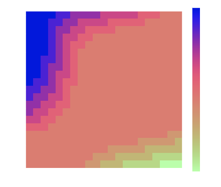
return new_policydef plot_policy(policy):
A = np.arange(0, MAX_CAPACITY+1)
B = np.arange(0, MAX_CAPACITY+1)
A, B = np.meshgrid(A, B)
Po = policy.reshape(MAX_CAPACITY+1,-1)
levels = range(-5,6,1)
plt.figure(figsize=(7,6))
CS = plt.contourf(A, B, Po, levels)
cbar = plt.colorbar(CS)
cbar.ax.set_ylabel('actions')
#plt.clabel(CS, inline=1, fontsize=10)
plt.title('Policy')
plt.xlabel("cars at B")
plt.ylabel("cars at A")Q-Function
The action-value function \(q_\pi (s,a)\) of an MDP is the expected return starting from state \(s\) with action \(a\), and then follow policy \(\pi\)
\[ q^\pi (s,a) = \mathbb E_\pi[G_t \mid S_t=s, A_t=a] \]
Optimal action-value function
\[ q^* (s, a) = \max_\pi q^\pi(s, a) \]
The optimal action-value \(q^*(s, a)\) of state-action pair \((s,a) \in \mathcal S \times \mathcal A\) gives the highest achievable expected return when the process is started from state \(s\), and the first action chosen is \(a\). The function \(q^* : \mathcal S \times \mathcal A \rightarrow \mathbb R\) is called the optimal action-value function.
Connection between optimal value- and action-value function
\[ v^*(s) = \max_{a \in \mathcal A} q^*(s,a), s \in \mathcal S \]
\[ q^*(s,a) = \mathcal R_s^a + \gamma\sum_{s' \in \mathcal S} P(s,a,s')v^*(s'); s \in \mathcal S, a \in \mathcal A \]
Bellman Equation for Q
\[ q_\pi(s, a) = \mathcal R_s^a + \gamma \sum_{s' \in \mathcal S} \mathcal P^a_{s,s'} \left( \sum_{a'\in \mathcal A} \pi(a' \mid s') q_\pi(s',a') \right) \]
for a deterministic policy:
\[ q_\pi(s, a) = \mathcal R_s^a + \gamma \sum_{s' \in \mathcal S} \mathcal P^a_{s,s'} q_\pi(s',\pi(s')) \]
\[ \hat Q^\pi = \hat R + \gamma \mathcal P \vec Q^\pi_\pi \] with
- \(\vec \pi\): Policy vector
- Matrices \(\hat Q^\pi, \hat R\) with entries \(\cdot_{sa}\)
- 3d Array \(\mathcal P\) with entries \(\cdot_{sas'}\)
- \(\vec Q^\pi_\pi = \vec v^\pi\)
Policy Evaluation for Q
Computing the state-action-value function \(q^\pi(s, a)\) for an arbitrary policy by an iterative application of Bellman expectation backup is also called policy evaluation:
- \(q_1 \rightarrow q_2 \rightarrow q_3 \rightarrow \dots \rightarrow q_\pi\)
- using synchronous backups
- at each iteration \(k+1\)
- for all states \(s \in \mathcal S\) and \(a \in \mathcal A\)
- update \(q_{k+1}(s, a)\) from \(q_k(s', \cdot)\), where \(s'\) is a successor state of \(s\).
\[ \hat Q^{k+1} = \hat R + \gamma \mathcal P \vec Q^k_{k} \]
# Iterative update of the bellmann equation for Q
def evaluate_policy_Q_by_iteration(
  policy,
  Q = np.zeros([(MAX_CAPACITY+1) ** 2,
  2*TRANSFER_MAX+1])
):
    converged = False
    P_ = P.transpose(1,2,0)
    while not converged:
        policy_index = policy + TRANSFER_MAX
        Q_pi = Q[np.arange((MAX_CAPACITY+1)**2), policy_index]
        new_Q = Reward + GAMMA * np.dot(P_, Q_pi)
        if np.allclose(new_Q, Q):
            converged = True
        Q = new_Q
    return Q
Policy Iteration for Q
- Starting with an arbitrary policy
- Iteration until the values converge (to the optimal policy). Alternating sequence of
- Policy Evaluation : Compute the values of the policy
- Greedy Policy Improvement:
- \(\pi'(s) = \text{arg} \max_{a \in \mathcal A} q^\pi(s,a)\)
- Note: Here we don’t use the (transition) model.
def greedy_improve_Q(Q):
    return np.argmax(Q, axis=1) - TRANSFER_MAX


policy = np.ones((MAX_CAPACITY+1)**2, dtype=int) * 0
Q = np.zeros([(MAX_CAPACITY+1)**2, 2*TRANSFER_MAX+1])

converged=False
while not converged:
    new_Q = evaluate_policy_Q_by_iteration(policy, Q)
    policy = greedy_improve_Q(Q)
    if np.allclose(new_Q, Q):
            converged = True
    Q = new_Q
Bellman Optimality Equation
\[ \begin{aligned} v^*(s) & = \max_a \mathbb E \left[ R_{t+1} + \gamma v^*(S_{t+1}) \mid S_t = s, A_t = a \right] \\ & = \max_a \left( \mathcal R^a_{s} + \gamma \sum_{s'} P_{ss'}^a \mathcal v^*(S_{t+1}=s') \right) \end{aligned} \]
\[ \begin{aligned} q^*(s, a) &= \mathbb E \left[ R_{t+1} + \gamma \max_{a'} q^*(S_{t+1},A_{t+1}=a') \mid S_t = s, A_t = a \right] \\ &= \mathcal R^a_{s} + \gamma \sum_{s'} P_{ss'}^a \mathcal \max_{a'} q^*(S_{t+1}=s',A_{t+1}=a') \end{aligned} \]
Value Iteration
From the Bellmann optimality equation we can derive an iterative method to find the optimal value function:
\[ \begin{aligned} v_{k+1}(S_t = s) &= \max_a \mathbb E[R_{t+1} + \gamma v_k(S_{t+1}=s') \mid S_t=s, A_t=a] \\ & = \max_a \left( \mathcal R_{s}^a + \gamma \sum_{s'} \mathcal P_{ss'}^a v_k(s') \right) \end{aligned} \]