Finite Markov Decision Processes (MDPs)

That is what ChatGPT would answer to a 5-year-old kid. Alright, let’s imagine you have a little robot friend named Robo. Robo likes to explore and do different things, but Robo doesn’t always know what to do next. A Markov Decision Process (MDP) is like giving Robo a set of rules to help it decide what to do next based on where it is and what it knows.

Imagine Robo is in a room full of toys. Each toy is like a different choice Robo can make, like playing with blocks or reading a book. But Robo can’t see the whole room at once, so it has to decide what to do based on what it can see and remember.

In an MDP, Robo learns from its past experiences. If it finds that playing with blocks usually makes it happy, it’s more likely to choose that again next time. But if it tries reading a book and doesn’t like it, it might choose something else next time.

So, a Markov Decision Process helps Robo make decisions by learning from what it’s done before and what it can see around it, kind of like how you learn from playing with different toys and remembering which ones you like best.

The Agent–Environment Interface

Example 1 A mobile robot has the job of collecting empty soda cans in an office environment. It has sensors for detecting cans, and an arm and gripper that can pick them up and place them in an onboard bin; it runs on a rechargeable battery. The robot’s control system has components for interpreting sensory information, for navigating, and for controlling the arm and gripper. High-level decisions about how to search for cans are made by a reinforcement learning agent based on the current charge level of the battery. To make a simple example, we assume that only two charge levels can be distinguished, comprising a small state set \(\mathcal{S} = \{\texttt{high}, \texttt{low} \}\). In each state, the agent can decide whether to

1. actively search for a can for a certain period of time,
2. remain stationary and wait for someone to bring it a can, or
3. head back to its home base to recharge its battery.

When the energy level is high, recharging would always be foolish h, so we do not include it in the action set for this state. The action sets are then \(\mathcal{A}(\texttt{high}) = \{\texttt{search}, \texttt{wait}\}\) and \(\mathcal{A}(\texttt{low}) = \{\texttt{search}, \texttt{wait}, \texttt{recharge}\}\).

The rewards are zero most of the time, but become positive when the robot secures an empty can, or large and negative if the battery runs all the way down. The best way to find cans is to actively search for them, but this runs down the robot’s battery, whereas waiting does not. Whenever the robot is searching, the possibility exists that its battery will become depleted. In this case the robot must shut down and wait to be rescued (producing a low reward).

If the energy level is high, then a period of active search can always be completed without risk of depleting the battery. A period of searching that begins with a high energy level leaves the energy level high with probability \(\alpha\) and reduces it to low with probability \(1 - \alpha\). On the other hand, a period of searching undertaken when the energy level is low leaves it low with probability \(\beta\) and depletes the battery with probability \(1 - \beta\). In the latter case, the robot must be rescued, and the battery is then recharged back to high. Each can collected by the robot counts as a unit reward, whereas a reward of \(-3\) results whenever the robot has to be rescued. Let \(r_{\texttt{search}}\) and \(r_{\texttt{wait}}\), with \(r_{\texttt{search}} > r_{\texttt{wait}}\), denote the expected numbers of cans the robot will collect (and hence the expected reward) while searching and while waiting respectively. Finally, suppose that no cans can be collected during a run home for recharging, and that no cans can be collected on a step in which the battery is depleted. This system is then a finite MDP, and we can write down the transition probabilities and the expected rewards, with dynamics as indicated in the table on the left:

Figure 1: Recycling-robot’s graph. Taken from [@Sutton2018]

Figure 2

Goals and Rewards

In reinforcement learning, the reward hypothesis serves as the foundation for defining the objectives of an agent operating within an environment. According to this hypothesis, the agent’s goal can be represented by the maximization of the expected cumulative reward over time, based on scalar feedback signals received from the environment.

Key Points of the Reward Hypothesis:

1. Reward as a Scalar Signal: At every time step, the environment provides the agent with a simple numerical signal, \((R_t \in \mathbb{R}\), which represents the immediate reward based on the agent’s actions and the current state of the environment. This reward acts as feedback for the agent, helping it learn and adjust its strategy to achieve its ultimate goal.

2. Maximizing Cumulative Reward: The agent’s goal is not just to maximize the immediate reward, but to focus on the long-term sum of rewards, known as the cumulative reward. This ensures that the agent does not become short-sighted by only pursuing short-term benefits, but rather seeks strategies that maximize its total reward across time.

3. Expected Value of the Reward: Since reinforcement learning involves interaction in environments that can be stochastic (involving randomness or uncertainty), the agent aims to maximize the expected value of the cumulative reward, accounting for different possible future states and outcomes. This means the agent is interested in the average cumulative reward it would obtain over many possible sequences of interactions, rather than specific individual outcomes.

4. Formalizing Goals and Purposes: According to the reward hypothesis, all goals, objectives, or purposes of the agent can be quantified by maximizing this cumulative scalar signal (reward). In other words, the “purpose” of the agent is simply to optimize the feedback it receives in the form of rewards, and this concept encapsulates everything the agent is designed to achieve.

Importance in Reinforcement Learning:

This hypothesis is central to how reinforcement learning problems are structured. It reduces complex goals and objectives into a single, scalar value (the reward) that the agent can track and optimize over time. This abstraction makes it possible to design agents that can handle a wide variety of tasks, as long as those tasks can be expressed in terms of rewards provided by the environment.

Returns and Episodes

To formalize the objective of learning in reinforcement learning, we introduce the concept of return. The return, denoted \(G_t\), is a function of the future rewards that the agent will receive after time step \(t\). The agent aims to maximize the expected return to achieve its goal. Let’s break down this formalization step by step:

1. The Reward Sequence:

At each time step \(t\), the agent receives a reward \(R_{t+1}, R_{t+2},\dots,\) as a result of interacting with the environment. This sequence of rewards represents the feedback the agent receives over time based on its actions.

2. Defining the Return:

The return at time step \(t\), denoted \(G_t\), is the total accumulated reward from time step \(t\) onward. In reinforcement learning, the return can be defined in different ways, but it generally involves summing the future rewards, often discounted to account for the uncertainty or diminishing value of rewards received further in the future.

The undiscounted return would simply be the sum of all future rewards: \[ G_t = R_{t+1} + R_{t+2} + R_{t+3} + \cdots = \sum_{k=0}^{\infty} R_{t+k+1} \] This sum may be infinite if the task never ends, which can be problematic. Thus, in many cases, a discount factor is applied to weight future rewards less than immediate rewards.

Likewise if the MDP has finite horizont \(T\) then \[G_t = R_{t+1} + R_{t+2} + R_{t+3} + \cdots + R_{T}\]

3. Discounted Return:

To address this issue, we introduce a discount factor \(\gamma\), where \(0\leq \gamma \leq 1\). The discount factor controls how much emphasis is placed on future rewards. When \(\gamma\) is close to 1, future rewards are considered nearly as valuable as immediate rewards. When \(\gamma\) is closer to 0, the agent focuses more on immediate rewards.

The discounted return is defined as: \[ G_t = R_{t+1} + \gamma R_{t+2} + \gamma^2 R_{t+3} + \dots = \sum_{k=0}^{\infty} \gamma^k R_{t+k+1} \] Here, each future reward is multiplied by ( ^k ), where ( k ) is the number of time steps into the future. This ensures that the agent values immediate rewards more highly than rewards far into the future, which is often desirable in practical applications.

4. Maximizing the Expected Return:

Since the environment in reinforcement learning is often stochastic, the agent cannot guarantee a specific sequence of rewards, but it can aim to maximize the expected return. The expected return is the average return the agent would obtain by following a specific policy \(\pi\), which defines the agent’s behavior.

Formally, the agent’s objective is to maximize the expected return: \[ \mathbb{E}[G_t | \pi] = \mathbb{E}\left[\sum_{k=0}^{\infty} \gamma^k R_{t+k+1} \Big| \pi\right] \] where \(\pi\) is the policy being followed. This equation tells us that the agent should choose actions in a way that maximizes the long-term expected reward, considering both immediate and future rewards.

5. Two Types of Tasks:

• Finite-Horizon Tasks: These tasks have a fixed time limit, and the agent’s goal is to maximize the sum of rewards within that time limit. In such cases, the discount factor \(\gamma\) may not be necessary, and the return is just the sum of the finite rewards received before the task ends.
• Infinite-Horizon Tasks: In tasks that continue indefinitely, the discount factor \(\gamma\) ensures that the return remains finite by reducing the impact of rewards far into the future.

Conclusion:

Thus, in reinforcement learning, the agent’s formal objective is to maximize the expected return, \(\mathbb{E}[G_t]\), where the return \(G_t\) is the discounted sum of future rewards. The use of the discount factor \(\gamma\) helps the agent focus more on immediate rewards, while still considering future rewards to some degree. This formalization ensures that the agent’s behavior is guided not just by immediate rewards but by a balanced approach to long-term success.

Unified Notation for Episodic and Continuing Tasks

Policies and Value Functions

In reinforcement learning (RL), value functions play a central role in determining the effectiveness of an agent’s behavior by estimating “how good” it is for the agent to be in a particular state or perform a specific action. Here, “how good” is quantified by future rewards the agent expects to accumulate, which is also known as the expected return. The expected return typically refers to the sum of future rewards, discounted over time, that an agent can expect to obtain from a particular state or state-action pair.

Key Concepts:

1. Value Functions:

A value function is a mathematical function that estimates the future rewards expected when starting in a specific state or taking a particular action in a state. Two types of value functions commonly appear in RL:

State value function \((V)\)

This estimates the value of a state, which is the expected return starting from that state and following a certain policy thereafter. The state value function \(V^\pi(s)\) under a policy \(\pi\) represents the expected return starting from state \(s\) and following the policy \(\pi\) thereafter. Mathematically, it is defined as:

\[ V^\pi(s) = \mathbb{E}_\pi \left[ G_t \mid S_t = s \right] \]

where:

• \(G_t\) is the return from time \(t\), typically defined as the sum of discounted rewards: \[ G_t = R_{t+1} + \gamma R_{t+2} + \gamma^2 R_{t+3} + \dots = \sum_{k=0}^{\infty} \gamma^k R_{t+k+1} \]
• \(S_t\) is the state at time \(t\), and \(R_{t+1}\) is the reward received after transitioning from state \(S_t\) to \(S_{t+1}\).
• \(\gamma\) is the discount factor that determines the present value of future rewards, where \(0 \leq \gamma \leq 1\).

The goal is to calculate \(V^\pi(s)\), which gives the expected return if the agent starts in state \(s\) and follows policy \(\pi\).

Action Value Function \(q_{\pi}(s, a)\)

The action value function \(q_{\pi}(s, a)\) gives the expected return for taking action \(a\) in state \(s\) and then following the policy \(\pi\). It is defined as:

\[ q_{\pi}(s, a) = \mathbb{E}_\pi \left[ G_t \mid S_t = s, A_t = a \right] \] This function tells us how good it is to take a particular action \(a\) in a state \(s\), assuming we follow policy \(\pi\) afterwards.

This estimates the value of taking a specific action in a given state, which represents the expected return from that state-action pair, following a particular policy from that point onwards.

2.Expected Return:

• The expected return is the total amount of reward an agent can anticipate from a particular point in time, considering both immediate and future rewards, usually discounted by a factor \(\gamma\) (the discount factor). This discount factor weights the importance of future rewards relative to immediate rewards.

3. Policies:

• A policy \(\pi\) is the strategy or decision-making rule that defines the actions an agent will take in any given state. The value functions are always associated with a particular policy, meaning the future rewards depend on the actions dictated by the policy.

Value functions are thus dependent on the agent’s policy, which determines the sequence of actions that the agent will take as it interacts with the environment. Policies can be deterministic (where each state leads to a fixed action) or stochastic (where actions are selected according to a probability distribution).

4. Bellman Equations for \(V^\pi(s)\) and \(q_{\pi}(s, a)\):

To compute the value functions, we use the Bellman equation, which expresses the value of a state or state-action pair in terms of the immediate reward plus the discounted value of the next state.

For the state value function, the Bellman equation is:

\[ V^\pi(s) = \sum_{a} \pi(a \mid s) \sum_{s'} P(s' \mid s, a) \left[ R(s, a, s') + \gamma V^\pi(s') \right] \]

where:

• \(\pi(a \mid s)\) is the probability of taking action \(a\) in state \(s\) under policy \(\pi\),
• \(P(s' \mid s, a)\) is the probability of transitioning to state \(s'\) after taking action \(a\) in state \(s\),
• \(R(s, a, s')\) is the reward received when transitioning from \(s\) to \(s'\) after taking action \(a\).

For the action value function, the Bellman equation is:

\[ q_{\pi}(s, a) = \sum_{s'} P(s' \mid s, a) \left[ R(s, a, s') + \gamma \sum_{a'} \pi(a' \mid s') Q^\pi(s', a') \right] \] These equations give a recursive way of expressing value functions, which are central to many RL algorithms.

\(Q\)-Learning (Off-policy learning algorithm)

Q-learning is a model-free, off-policy algorithm that seeks to find the optimal action-value function \(Q^*(s, a)\), which represents the maximum expected return for taking action \(a\) in state \(s\) and following the optimal policy from that point onward.

The Q-learning update rule is:

\[ Q(s_t, a_t) \leftarrow Q(s_t, a_t) + \alpha \left[ R_{t+1} + \gamma \max_{a'} Q(s_{t+1}, a') - Q(s_t, a_t) \right] \]

Where:

• \(\alpha\) is the learning rate,
• \(R_{t+1}\) is the immediate reward,
• \(\gamma\) is the discount factor,
• \(\max_{a'} Q(s_{t+1}, a')\) is the maximum estimated value of the next state \(s_{t+1}\) over all possible actions \(a'\).

The key feature of Q-learning is that it is off-policy, meaning that the learning happens regardless of the policy the agent is currently following. The agent can learn the optimal policy while exploring the environment using a different policy.

Policy Iteration (On-policy learning algorithm)

Policy iteration is a classic on-policy algorithm that alternates between policy evaluation and policy improvement until the optimal policy is found.

• Policy Evaluation: Given a policy \(\pi\), calculate the value function \(V^\pi(s)\) for all states using the Bellman equation for the state-value function.

  This involves solving the system of equations for \(V^\pi(s)\) either by iterating until convergence (infinite horizon) or using a matrix form if the state space is small.

• Policy Improvement: Using the current value function \(V^\pi(s)\), improve the policy by choosing actions that maximize the expected return:

\[ \pi'(s) = \arg\max_a \sum_{s'} P(s' \mid s, a) \left[ R(s, a, s') + \gamma V^\pi(s') \right] \]

These two steps repeat: after improving the policy, we re-evaluate the value function and then improve the policy again. The algorithm converges when the policy no longer changes, indicating that the optimal policy \(\pi^*\) has been found.

Value Iteration

Value iteration combines policy evaluation and policy improvement into a single step. Instead of fully evaluating the current policy, value iteration updates the value function directly using the Bellman optimality equation:

\[ V(s) \leftarrow \max_a \sum_{s'} P(s' \mid s, a) \left[ R(s, a, s') + \gamma V(s') \right] \]

Once the value function has converged, the optimal policy \(\pi^*\) is derived by choosing actions that maximize the value function.

Summary:

In summary, value functions \(V^\pi(s)\) and \(q_{\pi}(s, a)\) estimate future rewards based on an agent’s policy. These functions are fundamental to algorithms like Q-learning (off-policy) and policy iteration (on-policy). Q-learning directly updates the Q-values, aiming to discover the optimal action-value function, while policy iteration alternates between evaluating a policy and improving it.

Pick and drop example

Pick and Drop game

Figure 4.1: Pick and Drop game. See python implementation below.

Rewards rules for the drop game

Figure 4.2: Rewards rules for the drop game. See the above scheme for reference.

We use the following class to simulate the pick and drop game accordingly the

above figure and rules.

pick_and_drop_game.py

class Field:
    def __init__(self, size, item_pickup, item_dropout, start_position):
        self.size = size
        self.item_pickup = item_pickup
        self.item_dropout = item_dropout
        self.position = start_position
        self.item_in_car = False
    
    def get_number_of_states(self):
        return self.size * self.size * self.size * self.size * 2
    
    def get_state(self):
        state = self.position[0] * self.size * self.size * self.size * 2
        state = state + self.position[1] * self.size * self.size * 2
        state = state + self.item_pickup[0] * self.size * 2
        state = state + self.item_pickup[1] * 2
        
        if self.item_in_car:
            state = state + 1
        return state
    
    def make_action(self, action):
        (x, y) = self.position
        if action == 0:  # down
            if y == self.size - 1:
                return -10, False
            else:
                self.position = (x, y + 1)
                return -1, False
        
        elif action == 1:  # up
            if y == 0:
                return -10, False
            else:
                self.position = (x, y - 1)
                return -1, False
        
        elif action == 2:  # left
            if x == 0:
                return -10, False
            else:
                self.position = (x - 1, y)
                return -1, False
        
        elif action == 3:  # right
            if x == self.size - 1:
                return -10, False
            else:
                self.position = (x + 1, y)
                return -1, False
        
        elif action == 4:  # pickup
            if self.item_in_car:
                return -10, False
            elif self.item_pickup != (x, y):
                return -10, False
            else:
                self.item_in_car = True
                return 20, False
        
        elif action == 5:  # dropout
            if not self.item_in_car:
                return -10, False
            elif self.item_dropout != (x, y):
                self.item_pickup = (x, y)
                self.item_in_car = False
                return -10, False
            else:
                self.item_in_car = False
                return 20, True

To illustrate how works this class

test_pick_and_drop_game.py

from pick_and_drop_game import Field
size = 10
item_pickup = (0, 0)
item_dropout = (9, 9)
start_position = (9, 0)



if __name__ == '__main__':
    field = Field(size, item_pickup, item_dropout, start_position)
    print(field.position)
    
# manual solution
field.make_action(2)
field.make_action(2)
field.make_action(2)
field.make_action(2)
field.make_action(2)
field.make_action(2)
field.make_action(2)
field.make_action(2)
field.make_action(2)
# pick
field.make_action(4)

field.make_action(0)
field.make_action(0)
field.make_action(0)
field.make_action(0)
field.make_action(0)
field.make_action(0)
field.make_action(0)
field.make_action(0)
field.make_action(0)

field.make_action(3)
field.make_action(3)
field.make_action(3)
field.make_action(3)
field.make_action(3)
field.make_action(3)
field.make_action(3)
field.make_action(3)
field.make_action(3)

field.make_action(5)

Now we implement a random but naive solution

pick_and_drop_naive_random_solution.py

from matplotlib import pyplot as plt

from pick_and_drop_game import Field
import random
import numpy as np


def random_solution():
    size = 10
    item_pickup = (0, 0)
    item_dropout = (9, 9)
    start_position = (9, 0)
    
    field = Field(size, item_pickup, item_dropout, start_position)
    
    done = False
    steps = 0
    
    while not done:
        action = random.randint(0, 5)
        reward, done = field.make_action(action)
        steps = steps + 1
    
    return steps


if __name__ == '__main__':
    steps = random_solution()
    print(steps)
    sampling_size = 100
    sample = [random_solution() for _ in range(sampling_size)]
    sample = np.array(sample)
    no_steps_mean = sample.mean()
    print('Mean of # steps for reach goal {:n}'.format(no_steps_mean))
    plt.show()

Next we apply the \(Q-\)learning algorithm for impove the above solution.

pick_and_drop_q_learning_solution.py

    def q_learning_solution():
    epsilon = 0.1
    alpha = 0.1
    gamma = 0.6
    
    field = Field(size, item_pickup, item_drop_out, start_position)
    done = False
    steps = 0
    
    while not done:
        state = field.get_state()
        if random.uniform(0, 1) < epsilon:
            action = random.randint(0, 5)  # Explore
        else:
            action = np.argmax(q_table[state])  # Exploit
        
        reward, done = field.make_action(action)
        
        new_state = field.get_state()
        new_state_max = np.max(q_table[new_state])
        
        q_table[state, action] = \
            (1 - alpha) * q_table[state, action] \
            + alpha * (
                    reward + gamma * new_state_max
                    - q_table[state, action]
            )
        steps = steps + 1
    return steps


size = 10
item_pickup = (0, 0)
item_drop_out = (9, 9)
start_position = (9, 0)

field = Field(size, item_pickup, item_drop_out, start_position)

number_of_states = field.get_number_of_states()
number_of_actions = 6
q_table = np.zeros((number_of_states, number_of_actions))
epsilon = 0.1
alpha = 0.1
gamma = 0.6
n_training = 100000
# Training phase

for _ in range(n_training):
    field = Field(size, item_pickup, item_drop_out, start_position)
    done = False
    while not done:
        state = field.get_state()
        if random.uniform(0, 1) < epsilon:
            action = random.randint(0, 5)  # Explore
        else:
            action = np.argmax(q_table[state])  # Exploit
        reward, done = field.make_action(action)
        new_state = field.get_state()
        new_state_max = np.max(q_table[new_state])
        # q_learning iteration as ascendant grad
        q_table[state, action] = \
            (1.0 - alpha) * q_table[state, action] \
            + alpha * (
                reward + gamma * new_state_max - q_table[state, action]
            )

q_learning_sampling = [q_learning_solution() for _ in range(10000)]
fig, ax = plt.subplots()
ax.hist(q_learning_sampling, bins=100)
ax.set_title('distribution of the No. of steps with the Q-Learning sol')
ax.set_xlabel('No. of steps')
ax.set_ylabel('Count')
fig.savefig("histogram_q_learning_solution.png")
plt.show()

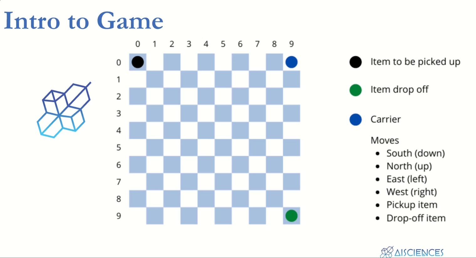
Example 4.1 (Gridworld)  

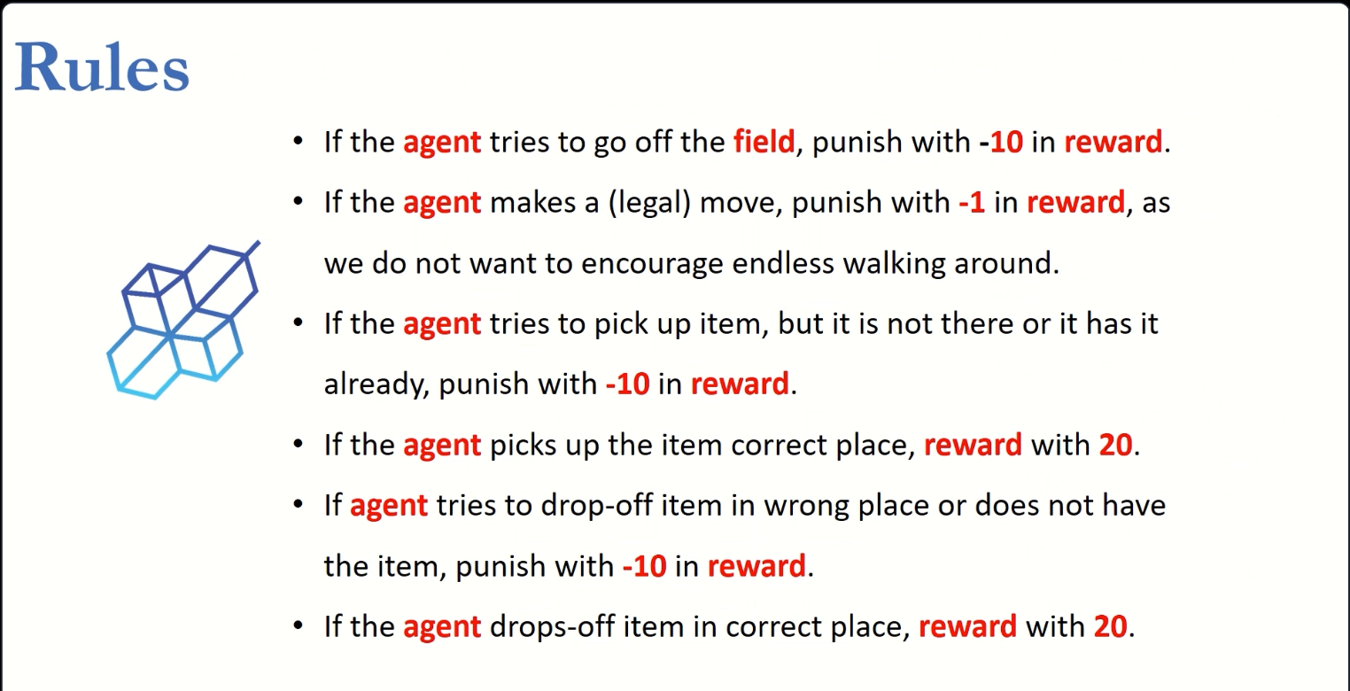
• Actions: north, south, east, west

• Rewards:

  • Actions would take the agent off the grid leave its location unchanged, but also results in a reward of-1;
  • Other actions result in a reward of 0, except those that in states A and B;
  • From state A , all four actions yield a reward of +10 and take the agent toA’ ;
  • From state B , all four actions yield a reward of +5 and take the agentto B’ ;
  • The learning rate (\(\gamma\)) for this example is 0.9

Grid World example. Problem scheme , possible actions and sampling reward

Figure 4.3: Grid World example. Problem scheme , possible actions and sampling reward

The Bellman equation must hold for each state for the value function \(v_{\pi}\) shown in Figure fig-grid-world-exm (right). Show numerically that this equation holds for the center state, valued at +0.7, with respect to its four neighboring states, valued at +2.3, +0.4, 0.4, and +0.7. (These numbers are accurate only to one decimal place.)

python implementation for the grid-world example

gridworld.py

#| lst-label: lst-import
#| lst-cap: Import pyplot
import matplotlib
import matplotlib.pyplot as plt
import numpy as np
from matplotlib.table import Table
matplotlib.use('Agg')

WORLD_SIZE = 5
A_POS = [0, 1]
A_PRIME_POS = [4, 1]
B_POS = [0, 3]
B_PRIME_POS = [2, 3]
DISCOUNT = 0.9

# left, up, right, down
ACTIONS = [np.array([0, -1]),
           np.array([-1, 0]),
           np.array([0, 1]),
           np.array([1, 0])]
ACTIONS_FIGS = ['←', '↑', '→', '↓']
ACTION_PROB = 0.25

def step(state, action):
    if state == A_POS:
        return A_PRIME_POS, 10
    if state == B_POS:
        return B_PRIME_POS, 5

    next_state = (np.array(state) + action).tolist()
    x, y = next_state
    if x < 0 or x >= WORLD_SIZE or y < 0 or y >= WORLD_SIZE:
        reward = -1.0
        next_state = state
    else:
        reward = 0
    return next_state, reward


def draw_image(image):
    fig, ax = plt.subplots()
    ax.set_axis_off()
    tb = Table(ax, bbox=[0, 0, 1, 1])

    nrows, ncols = image.shape
    width, height = 1.0 / ncols, 1.0 / nrows

    # Add cells
    for (i, j), val in np.ndenumerate(image):

        # add state labels
        if [i, j] == A_POS:
            val = str(val) + " (A)"
        if [i, j] == A_PRIME_POS:
            val = str(val) + " (A')"
        if [i, j] == B_POS:
            val = str(val) + " (B)"
        if [i, j] == B_PRIME_POS:
            val = str(val) + " (B')"
        
        tb.add_cell(i, j, width, height, text=val,
                    loc='center', facecolor='white')
        
    # Row and column labels...
    for i in range(len(image)):
        tb.add_cell(i, -1, width, height, text=i+1, loc='right',
                    edgecolor='none', facecolor='none')
        tb.add_cell(-1, i, width, height/2, text=i+1, loc='center',
                    edgecolor='none', facecolor='none')

    ax.add_table(tb)

def draw_policy(optimal_values):
    fig, ax = plt.subplots()
    ax.set_axis_off()
    tb = Table(ax, bbox=[0, 0, 1, 1])

    nrows, ncols = optimal_values.shape
    width, height = 1.0 / ncols, 1.0 / nrows

    # Add cells
    for (i, j), val in np.ndenumerate(optimal_values):
        next_vals=[]
        for action in ACTIONS:
            next_state, _ = step([i, j], action)
            next_vals.append(optimal_values[next_state[0],next_state[1]])

        best_actions=np.where(next_vals == np.max(next_vals))[0]
        val=''
        for ba in best_actions:
            val+=ACTIONS_FIGS[ba]
        
        # add state labels
        if [i, j] == A_POS:
            val = str(val) + " (A)"
        if [i, j] == A_PRIME_POS:
            val = str(val) + " (A')"
        if [i, j] == B_POS:
            val = str(val) + " (B)"
        if [i, j] == B_PRIME_POS:
            val = str(val) + " (B')"
        
        tb.add_cell(i, j, width, height, text=val,
                loc='center', facecolor='white')

    # Row and column labels...
    for i in range(len(optimal_values)):
        tb.add_cell(i, -1, width, height, text=i+1, loc='right',
                    edgecolor='none', facecolor='none')
        tb.add_cell(-1, i, width, height/2, text=i+1, loc='center',
                   edgecolor='none', facecolor='none')

    ax.add_table(tb)


def figure_3_2():
    value = np.zeros((WORLD_SIZE, WORLD_SIZE))
    while True:
        # keep iteration until convergence
        new_value = np.zeros_like(value)
        for i in range(WORLD_SIZE):
            for j in range(WORLD_SIZE):
                for action in ACTIONS:
                    (next_i, next_j), reward = step([i, j], action)
                    # bellman equation
                    new_value[i, j] += \
                        ACTION_PROB * (
                                reward + DISCOUNT * value[next_i, next_j]
                        )
                    
        if np.sum(np.abs(value - new_value)) < 1e-4:
            draw_image(np.round(new_value, decimals=2))
            plt.savefig('../images/figure_3_2.png')
            plt.close()
            break
        value = new_value

def figure_3_2_linear_system():
    '''
    Here we solve the linear system of equations to find the exact solution.
    We do this by filling the coefficients for each of the states with their respective right side constant.
    '''
    A = -1 * np.eye(WORLD_SIZE * WORLD_SIZE)
    b = np.zeros(WORLD_SIZE * WORLD_SIZE)
    for i in range(WORLD_SIZE):
        for j in range(WORLD_SIZE):
            s = [i, j]  # current state
            index_s = np.ravel_multi_index(s, (WORLD_SIZE, WORLD_SIZE))
            for a in ACTIONS:
                s_, r = step(s, a)
                index_s_ = np.ravel_multi_index(s_, (WORLD_SIZE, WORLD_SIZE))

                A[index_s, index_s_] += ACTION_PROB * DISCOUNT
                b[index_s] -= ACTION_PROB * r

    x = np.linalg.solve(A, b)
    draw_image(np.round(x.reshape(WORLD_SIZE, WORLD_SIZE), decimals=2))
    plt.savefig('../images/figure_3_2_linear_system.png')
    plt.close()

def figure_3_5():
    value = np.zeros((WORLD_SIZE, WORLD_SIZE))
    while True:
        # keep iteration until convergence
        new_value = np.zeros_like(value)
        for i in range(WORLD_SIZE):
            for j in range(WORLD_SIZE):
                values = []
                for action in ACTIONS:
                    (next_i, next_j), reward = step([i, j], action)
                    # value iteration
                    values.append(reward + DISCOUNT * value[next_i, next_j])
                new_value[i, j] = np.max(values)
        if np.sum(np.abs(new_value - value)) < 1e-4:
            draw_image(np.round(new_value, decimals=2))
            plt.savefig('../images/figure_3_5.png')
            plt.close()
            draw_policy(new_value)
            plt.savefig('../images/figure_3_5_policy.png')
            plt.close()
            break
        value = new_value


if __name__ == '__main__':
    figure_3_2_linear_system()
    figure_3_2()
    figure_3_5()

Example 4.2 The state is the location of the ball. The value of a state is the negative of the number of strokes to the hole from that location. Our actions are how we aim and swing at the ball, of course, and which club we select. Let us take the former as given and consider just the choice of club, which we assume is either a putter or a driver. The upper part of Figure shows a possible state-value function, \(v_{\text{putt}} (s)\), for the policy that always uses the putter.

Golf example

Figure 4.4: Gol example. At top the reward value of each state (ball curren position).

Optimal Policies and Optimal Value Functions

Optimality and Approximation

Summary

Bibliography